Comparing risk calculation models

Before 2008, the minimum capital requirements for market risk for financial institutions were calculated based on models using a plain Value at Risk (VaR) approach. Then the financial crisis hit markets in an unprecedented way, showcasing that many financial institutions were not sufficiently buffered with capital to withstand heavy market shocks.

This finding eventually pushed the Basel Committee on Banking Supervision to update and rewrite the regulations in place. FRTB (Fundamental Review of the Trading Book) is aiming to deliver a more robust framework targeting the minimum capital requirements for market risks, with the goal of shielding financial institutions from distress caused by coming crises. Among these renewals is the shift away from the predominant risk calculation method VaR to Expected Shortfall (ES).

As it measures the average losses that exceed the VaR level, ES is a risk measure that complements VaR. By using ES, financial institutions can obtain a more complete picture of the potential losses they could incur during adverse market conditions. Our analysis will compare the risk measurements of VaR and ES during the financial crisis of 2008, a period characterized by extreme market volatility and uncertainty, as well as during 2017, a period when quantitative easing was still in place, providing a more stable market environment. Ultimately, we aim to provide insights into the strengths and weaknesses of each approach in different market conditions.

Definitions

Before we take a look at the models’ performance under above-mentioned circumstances, we would first like to recall the definitions:

Value at Risk describes the maximum loss incurred in a predefined period of time and confidence level α.
An example use case within the FRTB framework involves measuring the risk to which a portfolio is exposed over a certain time period. For instance, the 10-day VaR at the 95% confidence level would offer the answer to the question: “What is the maximum loss amount that the portfolio will not surpass over a 10-day period with a probability of 95% ?”

Or in mathematical terms:
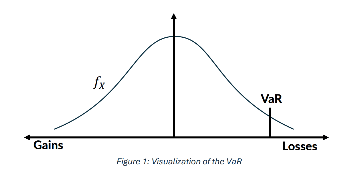
VaR is the 1–α percentile of the distribution function of losses over a certain period (see Figure 1):

where X is a random variable, F_X is the distribution function of losses during a 10-day period and α is the confidence level. f_x characterizes the density function of the loss amounts with the highest losses along the right tail and earnings (which are negative values since we are considering the loss function) along the left tail of the distribution.

The figure below shows a sample loss distribution function with the Value at Risk (VaR) marked on the right tail. VaR represents the maximum potential loss at a certain confidence level, with a probability of 1–α, where α is the chosen significance level.

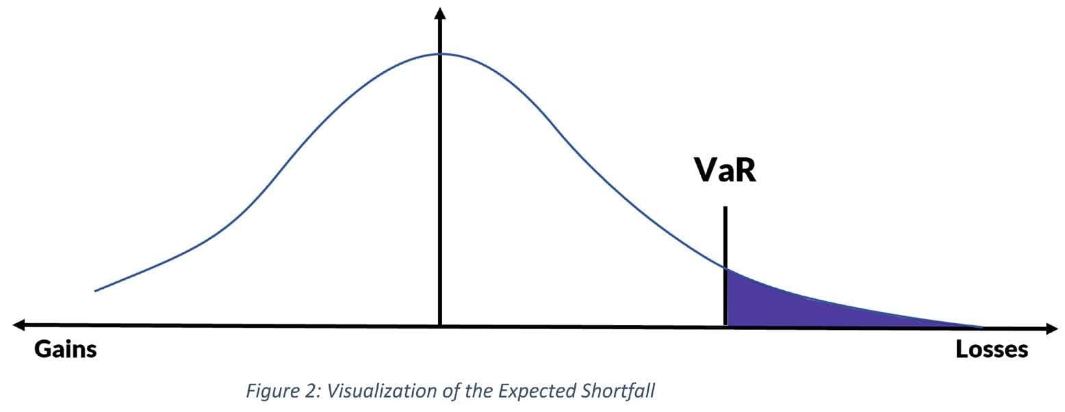
By contrast, Expected Shortfall measures the portfolio’s loss when it exceeds the limit set by VaR (see Figure 2). ES is the expected value of the loss, given the loss is greater than the VaR — or in other words it exceeds the (1–α)-percentile. Below it is visualized as the dark blue area under the distribution function.

In mathematical terms:

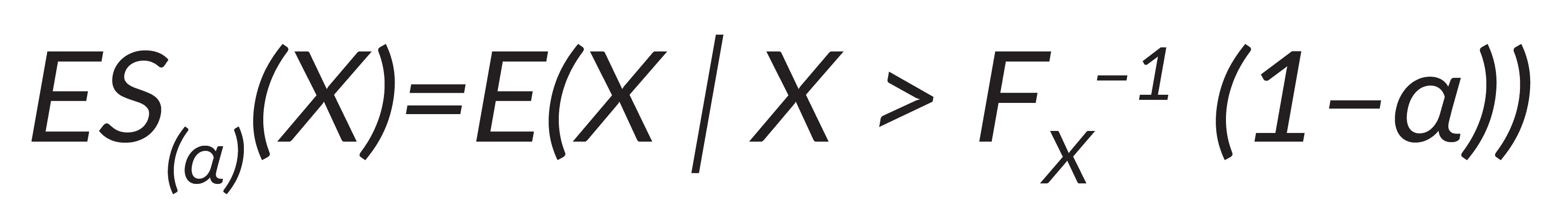
where X is a random variable and α expresses the confidence level.

Limitations and risks

When evaluating the accuracy of risk measures like Value at Risk (VaR) and Expected Shortfall (ES), it is important to keep in mind that they heavily rely on the underlying model for the loss distribution. These models can take different forms, such as historical data or derivatives of the normal distribution.

It is essential to acknowledge that these models may have limitations, particularly in accurately capturing tail risks. For instance, when using the normal distribution, tail risks may be underestimated, while historical data may not be an ideal representation of future data points, particularly along the tails of a distribution.
To ensure the accuracy of the risk measurement the model assumptions made when using VaR and ES should be carefully considered.

Furthermore, both VaR and ES are only capable of quantifying a subset of the risks faced by financial institutions. Other risks, such as liquidity, operational, and model risk, must also be considered when evaluating overall risk exposure.
While both are useful tools, they should be utilized in conjunction with other risk measures and frameworks to ensure a comprehensive risk management approach.

Case Study

Now that we are aware of the calculation methods and the peculiarities of our risk measures, we will have a closer look at how they behave under different market conditions to evaluate the impact on their outcome.

First, we will take a look at the period from April 2008 to April 2009. This is an exemplary period for severe levels of stress characterized by high volatility — owing to the financial crisis. This period is then contrasted with the period from January 2017 to December 2017. During this time span the European central bank was still pursuing its asset purchase program, representing a period of moderate market stress with relatively low volatility in the stock markets.

Visual Analysis:
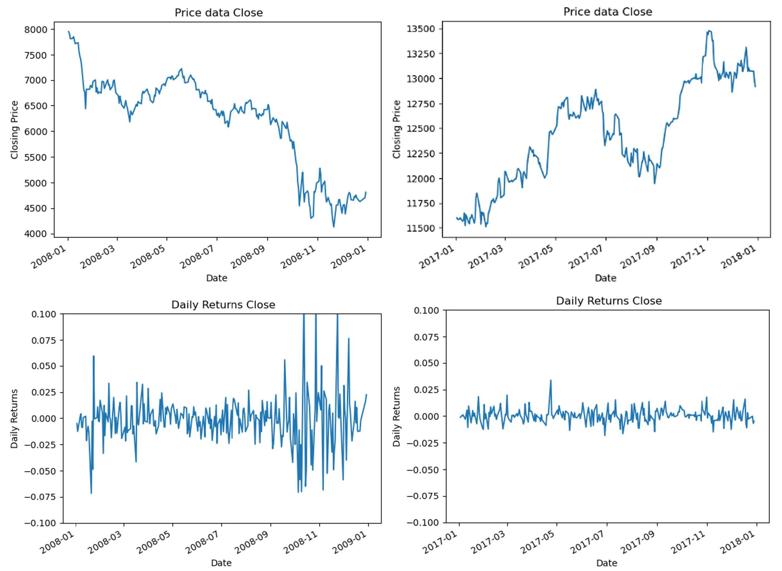
The first set of graphs illustrates DAX 30 Index’s values while the second set visualizes the DAX 30 day-to-day changes over the same period. At first glance, during the financial crisis we can observe rapid decreases of the index, also manifesting as large swings in the daily returns data. On some days even negative returns of -7 % were achieved.

On the contrary, the graphs on the right side depict a period of little market stress. The index is rising steadily and with much less volatility. The daily returns oscillate in a relatively narrow band around the zero percent line.

Computational Analysis:
Now, for a portfolio holding period of 10 days, we will calculate the average return as well as the VaR and the ES with a confidence level of 5% for each risk measure.
Assuming our portfolio’s initial value is 10,000$, we get our daily loss by multiplying the daily return value with the portfolio value at the market open. Since we are looking at the loss distribution, we must keep in mind, that amounts are positive while earnings are negative numbers.

We calculate the 95% percentile of our historical loss to determine the VaR for the confidence level of 5%. For the Expected Shortfall we first calculate the VaR for the given confidence level. In the second step, we determine the arithmetic mean over all the historical loss that surpassed this VaR.
In order to transform the risk measure we just calculated for a one day period into a 10-day period, we assume a normal distribution of our daily return values. This property allows us to get the desired 10-day risk measurement by multiplying the daily VaR by the square root of the number of days i.e. 10. The same applies for the ES.

Let’s have a look at the results in Figure 3:

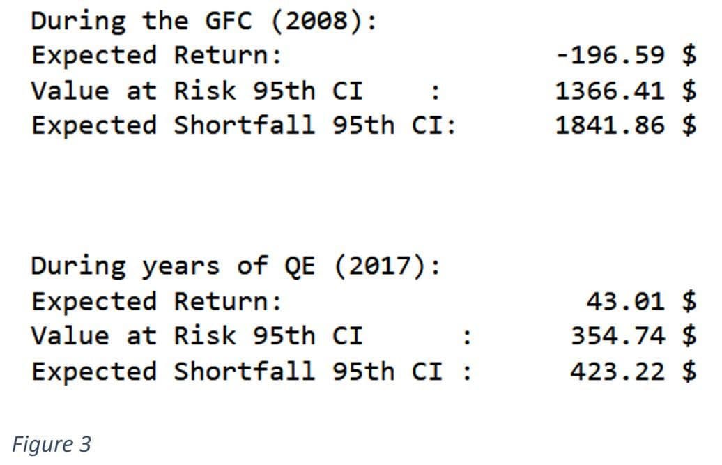
During the financial crisis of 2008, the portfolio’s expected return equaled -$196.59, indicating a substantial potential loss. The VaR, at a confidence level of 95%, was $1366.41, representing the maximum potential loss. However, the more comprehensive ES measure, which considers the severity of losses beyond the VaR, reached $1841.86.

These findings emphasize the significant risks and volatility that prevailed throughout the financial crisis. Both measures indicate potential losses, ES however provides an estimate of the expected shortfall, whilst VaR determines which loss amount will not be exceeded with a 95% confidence level.

In contrast, the portfolio’s predicted return improved to $43.01 during the 2017 period, suggesting a positive return expectation. The VaR at a 95% confidence level fell to $354.74, indicating a lower potential loss than in 2008. Similarly, the ES measure – condsidering the severity of losses – fell to $423.22.
These results point to a more stable and less volatile market environment in 2017, with lower potential losses compared to the financial crisis.

Conclusion

The comparison of these results demonstrates that ES provides valuable information in volatile market conditions. Unlike VaR, ES considers the severity of losses beyond the chosen confidence level, resulting in a more comprehensive risk assessment. ES emphasizes the possibility for more substantial losses during volatile periods such as the financial crisis, providing a deeper understanding of the portfolio’s downside risk. Further, even during periods of relative stability, such as 2017, ES still captures potential losses above and beyond the VaR. Since the volatility of the daily returns was lower, the values of both risk measures were closer to one another.

This historical example underscores the importance of adopting Expected Shortfall as a risk measure, particularly in volatile market conditions, as it provides more insights on potential losses than VaR. Nevertheless, keeping an eye on the model risks as well as the input data is critical when employing both measures to ensure good risk estimations.