
17.02.2026 / 08:30
The Unknown Pitfalls of Taylor Approximation in Energy Trading Valuation
Energy Markets

From quick estimates to costly errors: Understanding the pitfalls of Taylor approximations in energy risk management.

Taylor approximations are widely used in energy trading for their speed and simplicity. They enable near-real-time risk reporting and sensitivities, which is crucial for operational decision-making. However, when used as a substitute for full valuation, they can distort risk metrics, misprice convexity, and fail under stress – leading to implausible Value at Risk (VaR), misaligned hedges, and poor capital allocation.
Using the example of a gas swing contract, this article explains why the approximation fails for common energy structures, where the largest errors arise, and proposes full valuation as basis for more robust valuation and risk frameworks.
Nonexistent in the Banking Sector – Common in the Energy Sector
Taylor approximation can be a handy tool for risk management when it comes to the valuation of complex derivatives or products. Compared to a full revaluation, there is no need for expensive and time-consuming Monte Carlo simulations, as an approximation is usually ‘close enough’. By contrast, the front office in energy trading typically uses full valuation for pricing and PnL, as accuracy is critical for trading decisions.
In the banking sector, both front office and risk management usually employ full valuation for pricing and risk measurement. This is driven not only by the complexity of banking portfolios – often containing exotic derivatives and nonlinear payoffs – but also by regulatory requirements under Basel frameworks, which mandate accurate risk modeling for capital calculations, backtesting, and stress testing.
How Taylor Approximation Works
Taylor approximation is a mathematical technique used to approximate a complex function by a simpler polynomial, based on its derivatives at a specific point. It is widely used in energy trading to estimate changes in product values and risk metrics without performing full revaluation.
If you have a function V(x,σ) that is difficult to compute for every possible input, you can approximate it near a point (x₀, σ₀) using its derivatives at that point. For a product value V depending on prices x and volatility σ, the Taylor approximation is given by:
V(x, σ) ≈ V(x₀, σ₀) + Σᵢ Δᵢ (xᵢ − xᵢ₀) + 1/2 Σᵢⱼ Γᵢⱼ (xᵢ − xᵢ₀)(xⱼ − xⱼ₀) + ν (σ − σ₀)
Where:
Δᵢ = ∂V / ∂xᵢ : Delta – sensitivity to price changes
Γᵢⱼ = ∂²V / ∂xᵢ∂xⱼ : Gamma – curvature with respect to prices
ν = ∂V / ∂σ : Vega – sensitivity to volatility changes
The Taylor approximation is used because of its speed compared to full valuation. It also provides quick estimates of portfolio sensitivities and is easier to aggregate across positions. But it assumes small changes around the expansion point, and works best for smooth, linear functions. The approximation usually breaks down for non-linear, path-dependent, or discontinuous payoffs.
The calculation of Greeks, such as Delta, Gamma, and Vega, requires access to a full valuation model, because these sensitivities are derived from changes in the instrument’s value under small variations in market parameters. This full valuation model is typically developed and maintained for front office purposes to ensure accurate pricing and trading decisions.
Risk management leverages the same model to compute Greeks but does not use full revaluation for every risk metric. Instead, once the Greeks are calculated, risk teams apply Taylor approximations based on these sensitivities to estimate portfolio changes with reduced computational effort. Note that this approach also makes risk management dependent on front office models.
Risk Management is More than a VaR on Market Prices
While Taylor approximations can provide sufficiently accurate results for short-horizon risk metrics, such as VaR based on minor changes in market prices, they have significant limitations for other types of risk.
For example, in credit risk calculations, where exposures can change abruptly due to defaults, rating migrations, or counterparty events, the linear and quadratic assumptions underlying Taylor expansions often break down. This can lead to unstable and unreliable results, as approximations fail to capture discontinuities and nonlinear effects inherent in credit-sensitive instruments.
Therefore, while approximations are useful for speed in certain market risk contexts, they are generally unsuitable for metrics that involve structural changes or jump risks.
Example: Gas Swing Contract
The limitations of Taylor approximations become evident when applied to complex, highly nonlinear contracts such as a gas swing contract. These contracts allow the holder to vary daily or monthly gas offtake within predefined limits, creating significant optionality.
While a Taylor expansion based on Greeks may approximate small price movements reasonably well for short-term market risk metrics, it fails to capture the path dependency and embedded optionality inherent in swing contracts.
For example, changes in volatility or forward curve shape can drastically alter the optimal exercise strategy, leading to large valuation shifts that a Delta-Gamma approximation cannot predict. As a result, relying on approximations for such instruments can produce unstable and misleading risk figures, especially for metrics beyond short-horizon VaR, such as credit exposure or stress scenarios. This illustrates why full valuation is essential for complex energy derivatives.
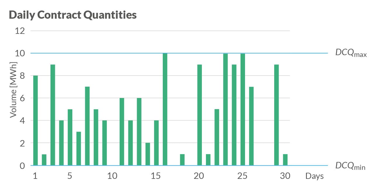
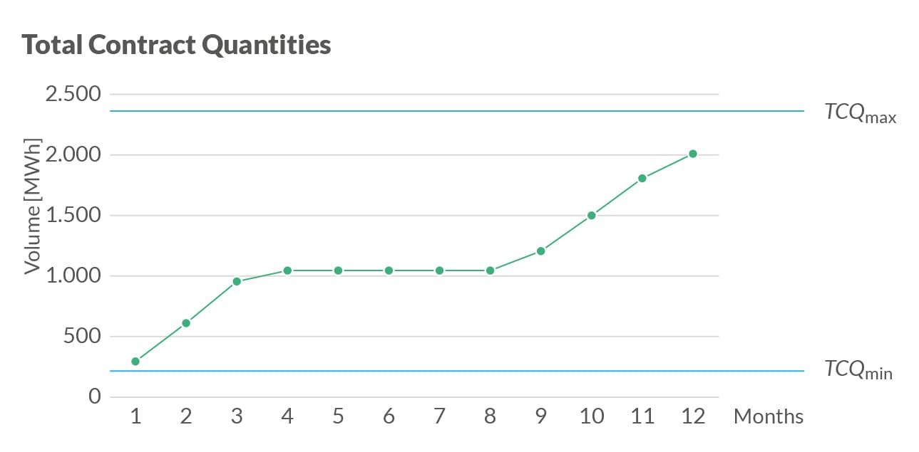
Figure 1: Illustrated Daily and Total Contract Quantities of the Gas Swing Contract, Including their Respective Boundaries
1. Contract Specifications
A long gas swing contract provides the option to buy gas daily for a fixed price, with some quantitative restrictions specified for the days, months, quarters, or the total contract period.
In the study below, the following gas swing specifications offer the daily option to buy a maximum of 10 MWh of gas. Furthermore, one needs to buy at least 240 MWh, and can, at most, buy 2,400 MWh per year. This results in a so-called daily contract quantity (DCQ) between DCQmin=0 and DCQmax=10, and a yearly or total contract quantity between TCQ TCQmin=240 and TCQmax=2,400.
2. Gas Spot Price Simulation via BM
In the following example, a spot model that is tied to a deterministic forward curve is used for the full valuation approach,
Spot(t) = Forward (t) + X(t)
where X(t) is an Ornstein-Uhlenbeck process (OU) of the form
dX(t) = κ(X(t) – θ)dt + σdW(t).
This OU process makes the spot process move randomly around the forward level in time. The volatility σ determines the size of the shocks generated by the random increments dW, whereas the mean reversion speed κ controls how fast the spot process moves back into the direction of the forward after a shock. The mean reversion level θ is typically set to 0 in the additive model, as defined above.
The described model is a common approach to spot modelling, also applicable in a logarithmic form, and can be easily extended with stochastic forward dynamics.
Figure 2 shows an example of a daily gas forward curve and its monthly average prices, together with simulations using the model described.
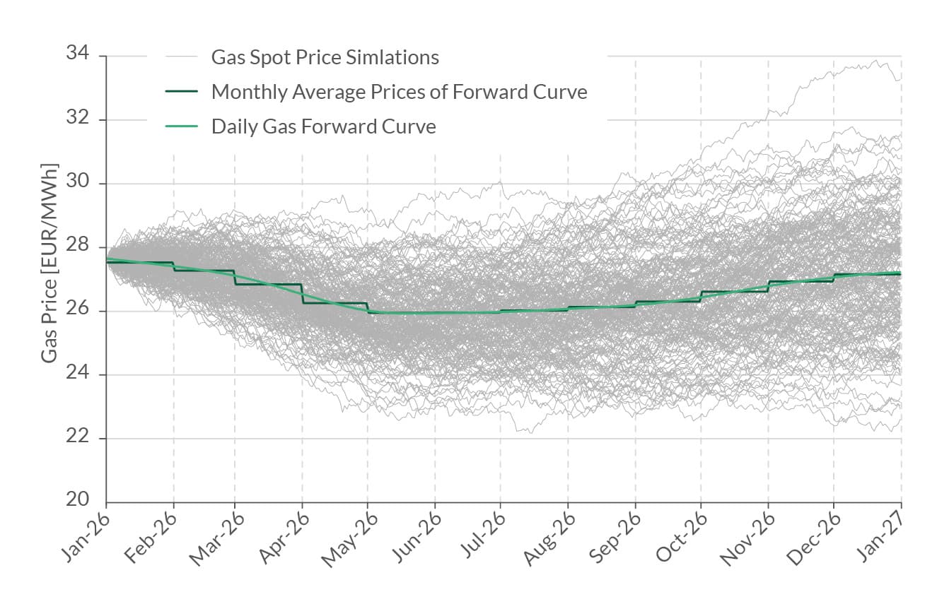
Figure 2: Gas Forward Curve and Simulated Spot Prices Based on the Forwards and the Described Model
3. Model for Full Valuation
Like other structured energy products, gas swings can be priced in different ways. The most common approaches – each offering greater flexibility but also requiring more computational effort – are analytical methods, numerical solutions of partial differential equations (PDEs), and Monte Carlo simulation techniques.
In this study, the PDE approach is used, since the gas swing option that is analyzed is of moderate complexity. A rough description of how the premium price is computed is given by the following steps:
The lifetime of the gas swing is discretized into days, as nominations are made on a daily basis as well.
The admissible volume levels and nomination volumes are determined and discretized in accordance with the imposed restrictions.
For each time and volume action, an expected value for the next time step can be formulated and calculated by solving a PDE. The model parameters described above are part of the matrices that define the PDE problem.
For the base scenario forward curve and valuation date 31st of December 2025, the full valuation price is 583.75 EUR. The Deltas and Gammas are computed using finite differences, first for a shift in the yearly price, then separately for each month within the swing period. The Vega is calculated only on a yearly basis, as it is less sensitive to temporal granularity. The exact numbers are displayed below in Table 1.
The monthly and daily Deltas in relation to the cumulated minimum and maximum volumes given by the restriction are shown in the upper part of Figure 4. Only the days from January to March and from November to December are in-the-money, relative to the contract price of 27 EUR.
Consequently, the maximum admissible daily gas volume is nominated at the beginning and end of the swing period. The daily Deltas flatten during days when the forward price is at-the-money and approach zero in summer, when market prices are low.

Table 1: Monthly Aggregated Spot Greeks for the Gas Swing Contract
4. Pricing under Market Shock Scenarios
Two plausible market shock scenarios are considered:
1. The first reflects an increase in the forward prices at the short end (Winter 2026) with a smaller price increase in later maturities. A rationale for this scenario could be an unusually cold winter, or lower-than-expected gas storage levels.
2. The second scenario builds on the first, but includes an upward shift of the entire forward curve by several euros. Such price changes could stem from geopolitical tensions or military conflicts. In the last years, the continental gas markets have been exposed several times to daily jumps of at least that size.
In both scenarios, the volatility is assumed to have doubled. Both market shock scenarios are shown in Figure 3.
Table 2 shows for scenario 1 the Taylor approximated gas swing prices, using the yearly spot Greeks as well as the monthly ones (the yearly Vega is used in both cases). Comparing those to the full valuation price, the relative error is 13% for using monthly spot Greeks and -11% for yearly ones, respectively.
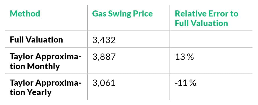
Table 2: The Taylor Approximated Gas Swing Prices for Scenario 1
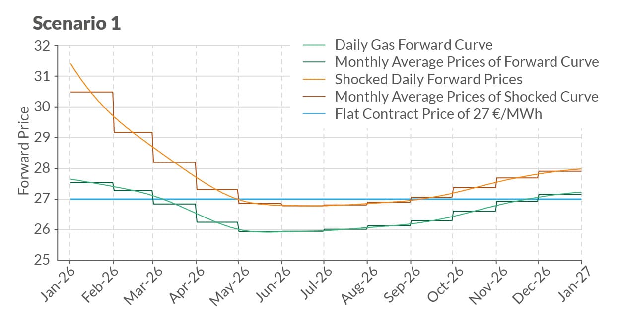
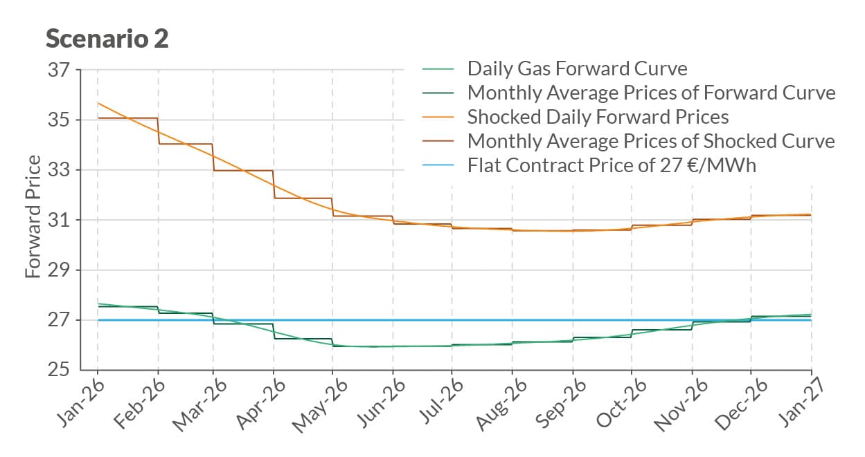
Figure 3: Shocked Forward Curve Scenarios
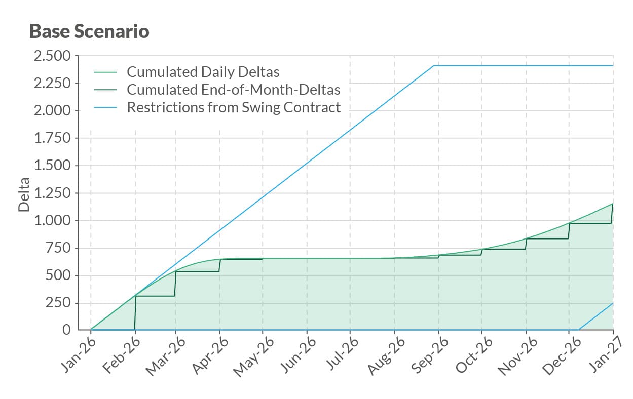
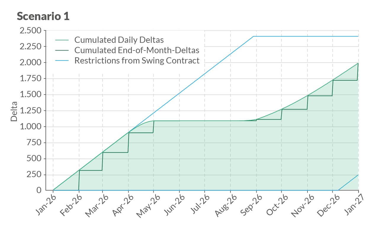
Figure 4: Delta and Volume Restrictions
As can be seen in the lower part of Figure 4, the daily and monthly Deltas derived from the full valuation approach using PDEs now extend into the summer. However, since the forward prices from May to August remain out-of-the-money, the cumulated Delta increase during these months is smaller.
For scenario 2, the Delta-Gamma-Vega approximation no longer works. The Deltas in the base case are too low, as a sizable portion of the forward prices in spring, summer, and autumn were out-of-the-money at that time. For those months in spring and autumn that were near the contract price, the Gamma was particularly high, causing the approximation to get too high as well. Table 3 displays the comparison of Taylor approximation against the full valuation price in scenario 2.
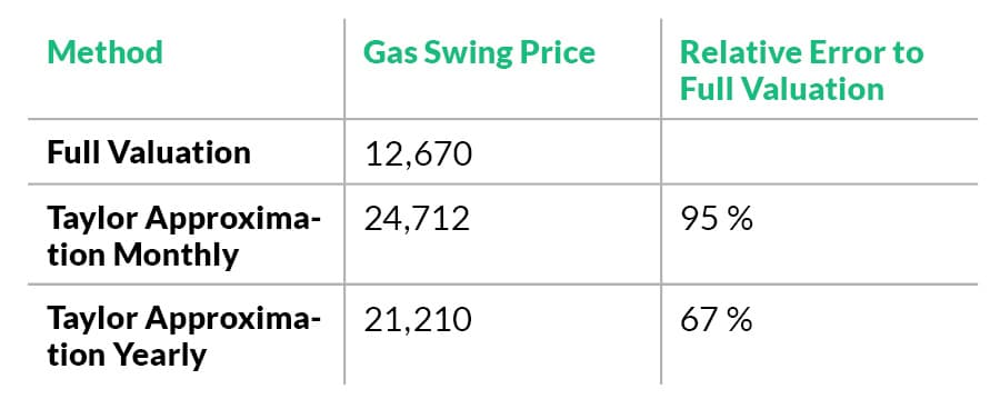
Table 3: The Taylor Approximated Gas Swing Prices for Scenario 2
Taylor Comes with Unmanaged Risk
As one can clearly see in our model results, a valuation with Taylor approximation can significantly differ from full valuation. This means companies that are using Taylor approximations are not accurately measuring their risk, and may make wrong decisions based on those results.
To overcome this, we strongly recommend changing risk valuation of all products and derivatives to a full valuation approach. The energy market is growing rapidly, with special emphasis on quick decision‑making. Those decisions need to be based on reliable and stable risk metrics.
Taylor approximation is a powerful analytic lens, but a fragile proxy when used as a wholesale replacement for valuation in energy trading. The technique’s local, smooth, small-move assumptions clash with the industry’s reality: nonlinear payoffs, regime changes, path dependence, and correlation dynamics. The results are implausible risk metrics when you need reliability most.